About this post

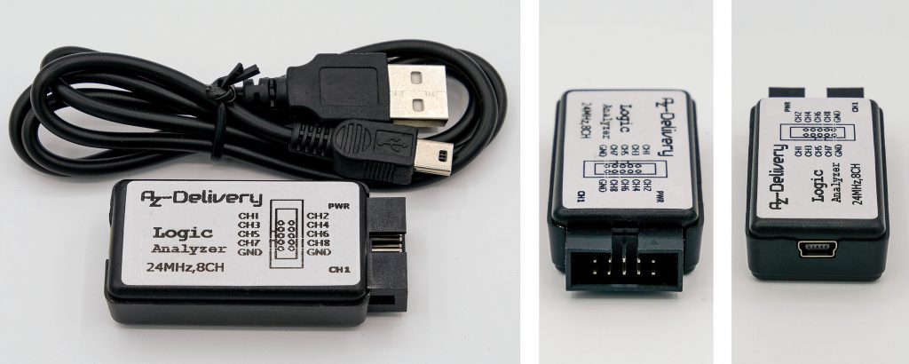
In this article I will introduce the 8-channel 24 MHz Logic Analyzer and the Logic 2 software. After hearing a lot about it, I recently took a closer look – and I really like it. Especially for troubleshooting and analyzing data transmissions, I find the device extremely useful.

This is what you can expect:

• Logic Analyzer – Basics and Properties
• Logic 2 – Overview
• Looping, Timer and Trigger measurements
  • looping
  • timer
  • trigger
• analyzer
  • async serial
  • I2C
• export analyzer data
• export raw data
• Other applications: 433 MHz and IR signals

Logic Analyzer – Basics / Properties

What does a Logic Analyzer do? In short, a logic analyser checks with a certain frequency whether a connected contact (e.g. a pin or a line) is at a HIGH or LOW level. You can think of it like an oscilloscope that only detects the logical states HIGH and LOW. The data is streamed via USB and analyzed by software. However, there are also PC-independent units that contain a display and control unit. 

The measurement frequency of the Logic Analyzer must be several times the frequency of the signals to be measured. For this article, I use one of the common, inexpensive logic analyzers that are available from as little as €10 on Amazon or other online shops. With its measuring frequency of 24 MHz, it is sufficient for most applications in the field of microcontrollers.

As for the voltage of the logic levels, I have found different information. The limit up to which LOW signals are reliably recognized as LOW seems to be somewhere between 0.6 and 1.0 volts. For the lower limit of the HIGH range, the specifications were between 1.2 and 1.8 volts. I cannot say whether the devices are actually different or just the information provided by the suppliers. They are therefore in any case suitable for the common 5 and 3.3 volt based microcontrollers.

For devices with higher measuring frequencies, you have to spend considerably more money. At Saleae you can get logic analysers that scan at 100 or 500 MHz, but they cost a few hundred to over a thousand euros.

The software I use is the free Logic 2 from Saleae. You can download the program here. The installation is so simple and unproblematic that I won’t go into it in detail. After installation, connect the Logic Analyzer to the PC, and it will be recognized immediately. At least that was the case with me.

An attentive reader has pointed out that the licence conditions do not allow Logic 2 to be used with devices from other manufacturers, although it works perfectly! The notice is quite well hidden. I would like to at least mention this. So you would either have to buy a Logic Analyser from Saleae or get an alternative software to avoid violating it.

Logic 2 – first overview

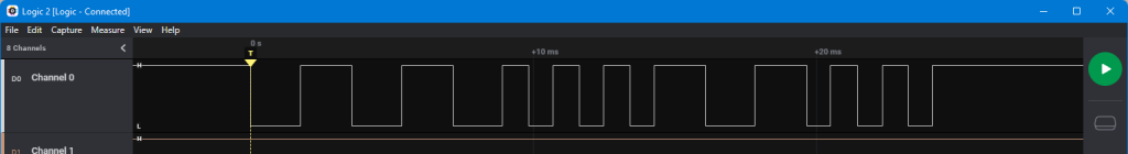
After you have installed Logic 2, connect the Logic Analyzer to the PC and launch the programme. Here is an overview:

1. Logic 2 window: Logic Analyzer connected or disconnected
2. Main menu
3. Timeline, scalable with +/- or mouse wheel
4. Channels 0 – 7
5. Start / Stop Button
6. Side menu
7. Device Settings: Logic Analyzer Settings
8. Analyzer: Activation of analysis programs
9. Timing Markers, Measurements & Notes: Evaluation of measurements
10. Extensions: Installable add-ons
11. Communication: click here to access the forum and support
12. Alternative to the main menu
13. Sessions: very convenient to switch between different sessions with different settings

You may have noticed that the channels in Logic 2 are numbered from 0 to 7. On the other hand, they are labeled 1 to 8 on the Logic Analyzer. But it’s just a shift by 1 channel. Channel 1 of the Logic Analyzer is channel 0 in Logic 2, etc.

Looping, Timer and Trigger measurements with the Logic Analyzer

There are three methods to control the timing of the measurements:

• Looping: the measurement is started manually and runs endlessly until it is stopped manually. The measured values are stored in a buffer. When the buffer is full, the oldest values are deleted in favor of new values.
• Timer: again, you start the measurement manually, but set the duration.
• Trigger: in this method – similar to interrupts – you set an event by which the measurement is started. This could be, for example, a LOW-HIGH change (rising edge). You can freely select the measurement duration.

Looping measurements

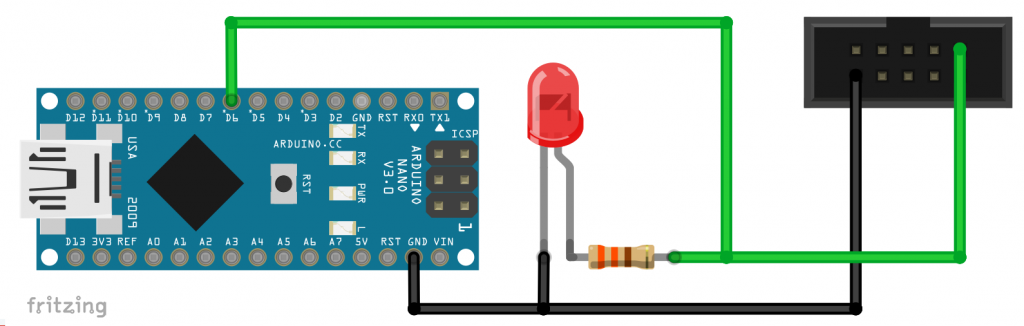
As a first example, let’s look at a constant PWM (pulse width modulation) signal generated with an analogWrite() statement. This signal is used to set an LED to a certain brightness. I chose an Arduino Nano as the MCU board. Here is the short sketch:

const int analogWritePin = 6;

void setup() {
  pinMode(analogWritePin, OUTPUT);
  analogWrite(analogWritePin, 51);
}

void loop() {}

 

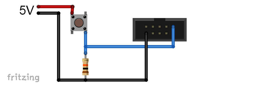
And now to the circuit. Basically, you need a common GND. There are two GND pins on the logic analyzer, which I symbolize here by the socket. We record the PWM signal with pin 1 of the Logic Analyzer.

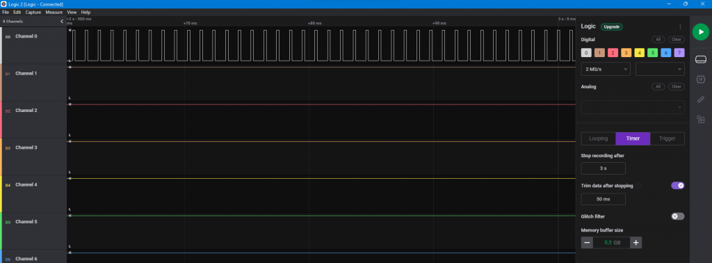
Since the signal is permanently present, we can use the looping method. To do this, go to the Device Settings in the side menu and select “Looping”. I set 2 MS/s (= 2 million samples per second) as the measuring frequency. Since the PWM frequency is about 1 kHz, I could have chosen a significantly lower value.

With “Trim data after stopping” you can reduce the collected data to a certain period of time.

The “glitch filter” eliminates noise signals. You recognize glitches as signals with a strikingly short duration. If this occurs, then you can activate the filter for the channel in question. You can set a time limit. All signals with a shorter duration are filtered out.  

The “Memory buffer size” determines how much RAM may be used as buffer memory. If the buffer is full, the oldest data is deleted from the buffer.

Now is the time: Click on the Start button and then – whenever you want – on Stop. Then move the mouse to the result of channel 0 and set the desired scaling with the mouse wheel. If you hold down the left mouse button, you can shift the curve.

When you move the mouse over the result curve of channel 0, the signal distances, the PWM frequency and the duty cycle are automatically displayed. As expected, the latter is 20 percent.

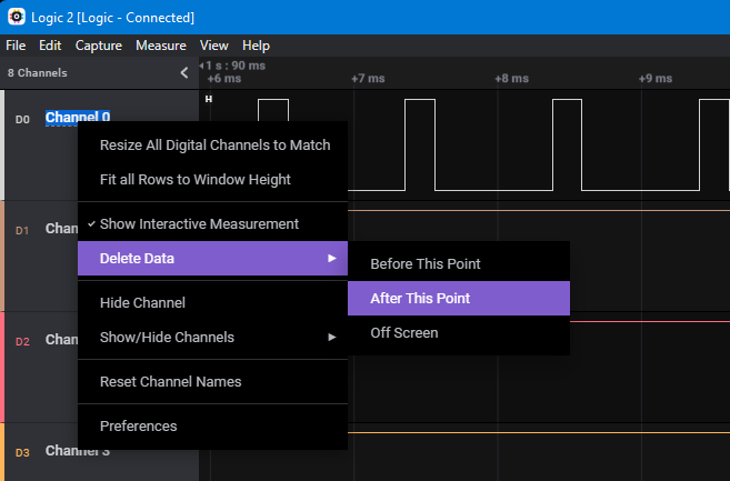
Deleting measured data

If you want to delete data, then right-click at a reference point, go to “Delete” and select your option.

Timer measurements

The timer method is useful, for example, if you want to determine the number of events in a certain period of time.

You set the length of a timer measurement with “Stop recording after”. For the result shown below, I have activated the option “Trim data after recording” and set it to 50 milliseconds. I didn’t change the circuit and the sketch.

Trigger measurements

The trigger method is suitable for individual events and especially if you do not know exactly when they occur. With “Pattern and Channel” you define the trigger and set the channel. The trigger can be a rising or falling edge, a HIGH pulse or a LOW pulse. You also determine the duration of the measurement.

Trigger Example 1: Push-Button

As a first example, I connected a push-button to the Logic Analyzer. In normal state it delivers a LOW to channel 0, when pressed it delivers a HIGH:

I have set a rising edge as the trigger. The measuring time after the trigger signal occurs is 5 seconds. I set the data acquisition to start 500 milliseconds before the trigger signal (“Trim pre trigger data”). During the 5 seconds, I pressed the button a few times:

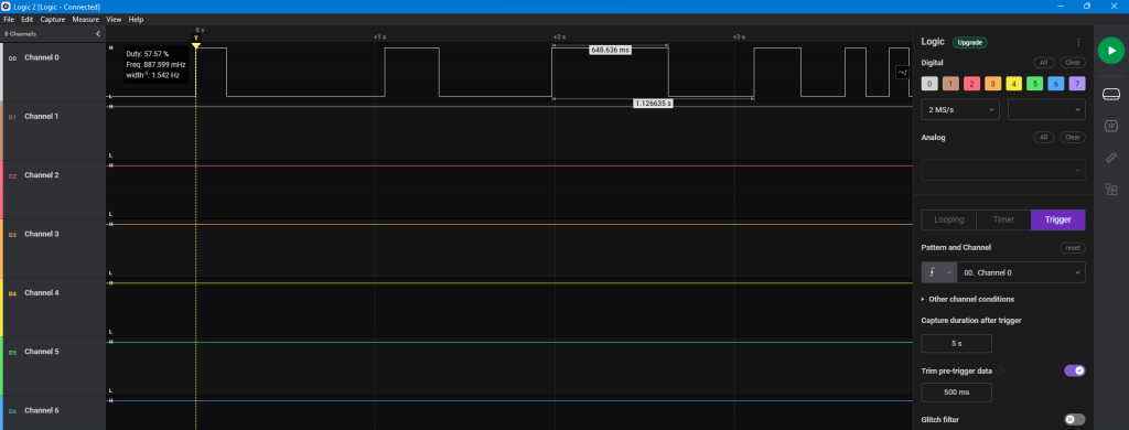
Admittedly, the example is rather pointless – but it shows the principle.

Trigger Example 2: HC-SR04

The next example makes a little more sense. Here I am examining what happens during a distance measurement with the HC-SR04. This is the circuit:

The trigger line is monitored with channel 0, the echo line with channel 1.

This is the sketch:

int triggerPin = 12;
int echoPin = 11;

void setup(){
  pinMode(triggerPin, OUTPUT);
  pinMode(echoPin, INPUT);
  Serial.begin(9600);
  delay(30);
}

void loop(){
  digitalWrite(triggerPin, HIGH);
  delayMicroseconds(20);
  digitalWrite(triggerPin, LOW);
  unsigned long duration = pulseIn(echoPin, HIGH);
 
  int cmDistance = duration * 0.03432 / 2; 
  Serial.print("Distanz [cm]: ");
  Serial.println(cmDistance);
  
  delay(3000);
}

 

I have set a rising edge as the trigger. The trigger signal for the HC-SR04 module is also the trigger for the Logic Analyzer. This is what a measurement in Logic 2 looked like (about 20 cm distance):

You can see how – after the short trigger signal and a certain latency – the echo pin goes to HIGH level and then back to zero when the echo is received. To determine the duration of latency, I set markers. This function can be found in the main menu under “Measure”. So the trigger signal is 22.25 microseconds and the latency is 443.75 microseconds.

However, this can be displayed even more clearly. For this purpose, there are “Measurements”, which you can access via the ruler symbol in the side menu. Click the “+” icon, and then click “Add Measurement”. If you then point the mouse at the result curve, a vertical red line appears which you can move and which snaps into place at markers and signal edges. After a left click, you can define the measuring range. It may sound complicated, but it’s simple and intuitive.

You can give the measuring ranges names and color them differently:

Analyzers

Now we move on to a really useful function, the so-called analyzers. This allows you to analyze the I2C, SPI or serial communication of your microcontroller with other components.

You activate the analyzer via the “1F” icon in the side menu. Then choose I2C, SPI or Async Serial. Depending on the selection, you have to make further settings.

Analyzer Example 1: Async Serial / SoftwareSerial

First, let’s look at serial communication using the example of a SoftwareSerial connection. Download the following SoftwareSerial sketch to your board.

#include <SoftwareSerial.h>
SoftwareSerial mySerial(10,11);

void setup() {
  Serial.begin(9600);
  Serial.println("Let's start!");
  mySerial.begin(9600);
}

void loop() { // run over and over
  if (mySerial.available()) {
    Serial.write(mySerial.read());
  }
  if (Serial.available()) {
    mySerial.write(Serial.read());
  }
}

 

You connect the TX pin (here: pin 11) to the Logic Analyzer. Of course, you must not forget the GND connection.

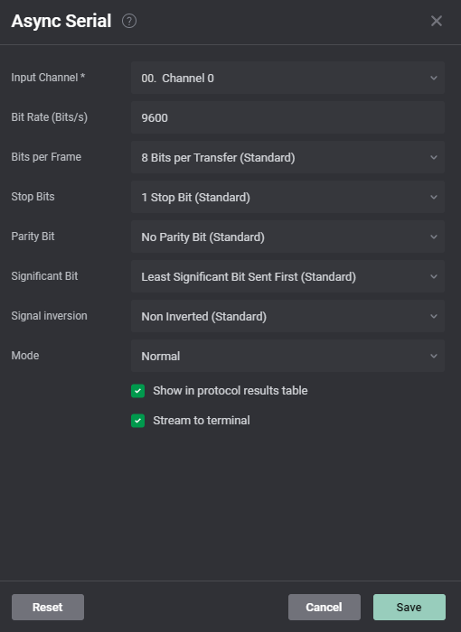
Now select “Async Serial”, whereupon a window opens with the details of the serial connection. Set the input channel and the baud rate you set. Normally, the other settings do not need to be changed. We will come to the options “Show in protocol results table” and “Stream to terminal” later.

For my example, the trigger method makes sense.

Since TX is usually HIGH and the signals are LOW, you should choose falling edge as a trigger. By the way, I did that wrong below, but then left it that way to show what happens → the trigger is not at the beginning of the signal.

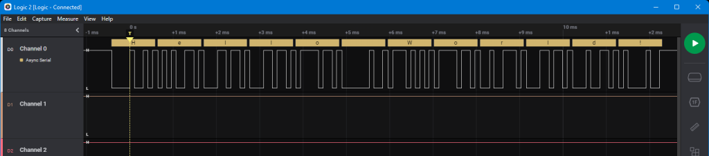
Start the measurement and open the serial monitor. Send any message. I took the good old “Hello World!” The trigger should start data acquisition. After the time you set, the measurement stops.

You will see that not only the signal, but also its meaning is displayed. By right-clicking on the bars above the signal, a selection menu appears in which you can choose between binary, decimal, hexadecimal and ASCII. Here’s what it looks like with ASCII:

You can see that the transmission of “Hello World” takes about 12 milliseconds at a baud rate of 9600. As expected, the process is correspondingly faster with 115200 BAUD:

If you want to repeat this yourself, don’t forget to change the baud rate in Logic 2 as well. This is what you do in the Analyzers section → the three dots behind “Async Serial” → Edit. There you also switch the analyser off again. If you forget this and carry out other measurements, you will get “frame errors”, which are noticeable by exclamation marks above the signals.

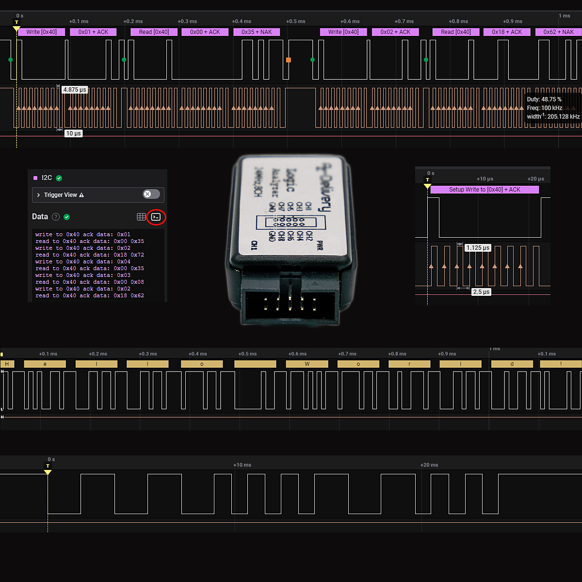
Analyzer Example 2: I2C

To try out the I2C Analyzer, take any I2C module and connect it to your microcontroller. Upload a suitable sketch that ensures communication between your microcontroller and the I2C component. I chose an INA219 current sensor and a sketch that regularly queries INA219 readings.

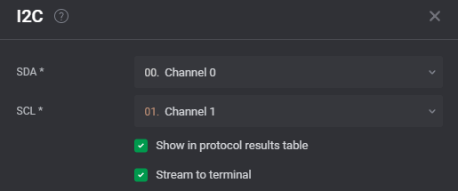
In Logic 2 you choose the Analyzer I2C. You will then be asked for the channels for SDA and SCL.  If not already done, connect the SDA / SCL lines to the selected channel pins.

For the control of the measurement, I would again choose the trigger mode so that I do not have to search for the signals in the recording. Since the I2C lines are HIGH in the ground state, the falling edge is again the trigger.

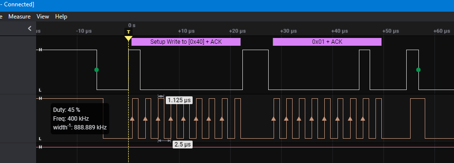
In my example, the INA219 module has the I2C address 0x40. The registers are 0x01 and 0x02 are read. Query and response are easy to track:

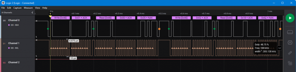
Here I have set the I2C frequency with setWireClock(400000) to 400 kHz:

As expected, the clock speed quadruples.

Export Logic Analyzer data

First of all, you can view the data evaluated by the analyzer, provided that you have set the previously mentioned but not explained ticks at “Show in protocol results table” and “Stream to terminal”. Here is the data in the terminal:

And here is the data in the data table:

To export the data, click on the three dots to the right of “Type to search”. Click on the columns you want to export and then go to “Export Table”.

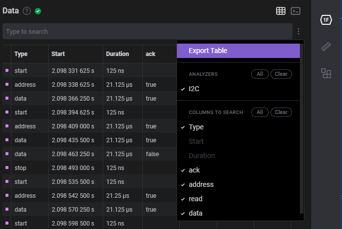
Another window will open where you can choose more options:

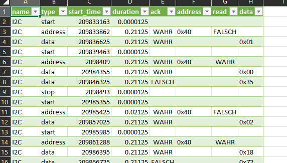
Now click on “Export”. You choose a file name and a directory for your “.csv” file and save it. Then you can import the file into Excel, for example to evaluate it statistically or to create graphics:

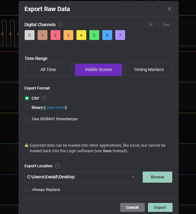
Export raw data

Alternatively, you can also export unevaluated raw data. These only contain the time and state of the selected channels. You can access the function via File → Export Data.

Other applications

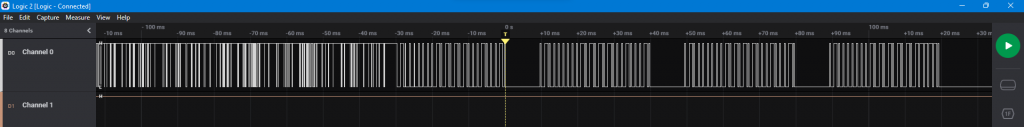
Analyze 433 MHz signals

In this example, I used the Logic Analyzer to capture a 433 MHz signal at the data output of a receiver. The signal was supplied by a remote control for a radio socket. The challenge is that the receiver without a “real” signal provides a lively data salad (see below, to the left of the trigger marker). Here it helped to select a LOW Pulse with a certain minimum width as a trigger.

Analyze IR signals

And finally, here is an IR signal that I generated with the remote control of my SAT receiver and captured with an IR receiver diode:

Here you can easily see the structure of the signal and could “recreate” the signal to simulate the remote control.