About the post

After recommending the DSO 138 oscilloscope in my last posts about timer (Part 1 and Part 2), I wanted to introduce it in a separate article. Some of you may have thought about buying an oscilloscope before, but then you’ve shied away from the high cost. With the DSO 138, however, there is a model that is available for less than 30 euros. From my point of view, it is a beautiful entry-level model that masters the basic functions of an oscilloscope.

This post is a mixture of user manual, product review and entry into the world of oscilloscopes. It is aimed primarily at those who have little to no experience with these devices.

What is an oscilloscope?

The core task of an oscilloscope is the display of signal voltages over time (YT mode). To provide stable images, oscilloscopes work with triggers, but I’ll come to that later. More expensive oscilloscopes have several signal inputs. The signals can then also be displayed against each other (XY mode) and no longer only over time. Usually multi-channel oscilloscopes can also process the signals mathematically, e.g. subtract them from each other. The DSO 138 has only one channel and therefore only masters the YT display.

Where can I get the DSO 138?

You can buy the DSO 138 in many online shops such as eBay, Amazon, AliExpress, Conrad, etc., in three variants:

• as a kit to be soldered
• ready for use
• ready for use with housing kit

The price depends on which variant you choose and how much delivery time you want to accept. But you should not pay more than 30 euros.

Specifications of the DSO 138

• Channels: 1 channel
• Bandwidth: 0 – 200kHz – put simply, this is the maximum frequency that can be recorded; if you want to know more, I recommend this article
• Sample Rate: 1 MSa/s
  • i.e. that 1 million times per second is sampled – this is rather the lower end in comparison; my “good” oscilloscope for just under 400 euros is capable of 1 GSa/s
• Maximum input voltage: 50 V pk (pk = peak, i.e. peak voltage)
• Input impedance: 1 MOhm / 20 pF – these are common values
• Resolution: 12 bits
• Recording length: 1024 points
• Time base range: 500 s/Div – 10 s/Div
  • this is the time per grid spacing on the display
• Trigger modes: auto, normal, single – is still explained
• Power supply: 9V DC (8-12Volt)
  • a power supply is not included
  • also works with a 9 V block in battery mode!
• Power consumption: approx. 120 mA
• Resolution TFT Display: 320 x 240 points

Controls

Simple buttons / sliders

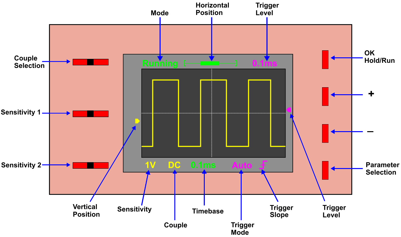
• Couple Selection: GND (separated from signal), AC (DC fractions are filtered out), DC (DC)
• Sensitivity 1: together with sensitivity 2 it determines how many volts correspond to the grid spacing; 1 V,   0.1 V or 10 mV
• Sensitivity 2: Factor 1, Factor 2 or Factor 5 for the range selected in Sensitivity 1
  • so you can set: 5 V, 2 V, 1V, 0.5 V, 0.2 V, 0.1 V, 50 mV, 20 mV and 10 mV
• OK/Hold/Run: stops the screen refresh; with another press, it continues; in keyboard shortcuts it is the OK key
• +/- : selected parameter larger or smaller
• Parameter selection:
  • Timebase: determines which time corresponds to the grid spacing
  • Trigger mode: auto, normal, single (will be explained in more detail)
  • Trigger slope: trigger is the falling or rising edge
  • Trigger level: trigger voltage level
  • Horizontal position: temporal scrolling through the signal
  • Vertical position: moves the baseline

Shortcuts

• Show measurement data on screen / deactivate (see next picture): select time base, then press OK for 2 seconds
• Save measurement: press select and “+” simultaneously
• View saved measurement: press select and “-” simultaneously

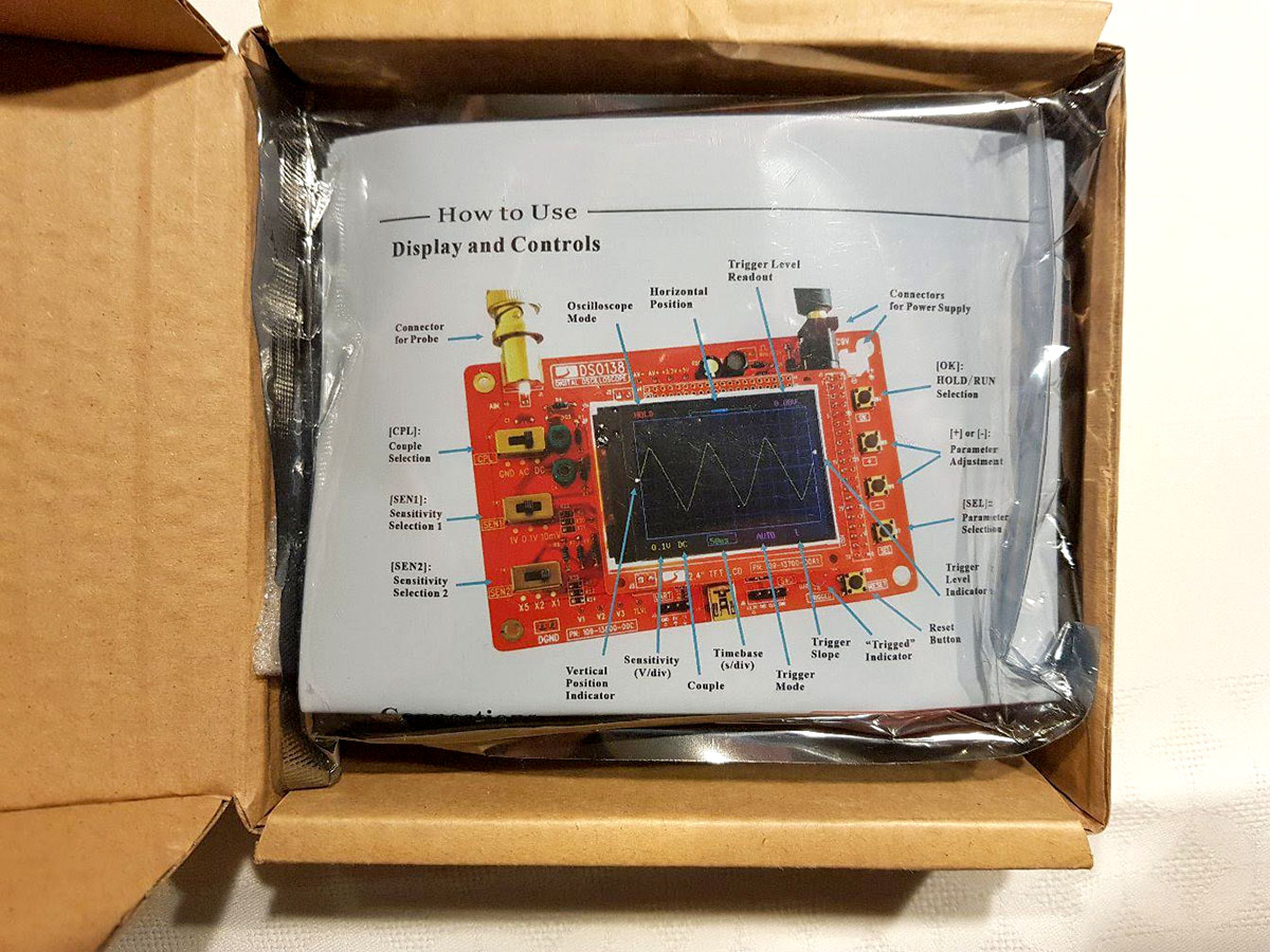
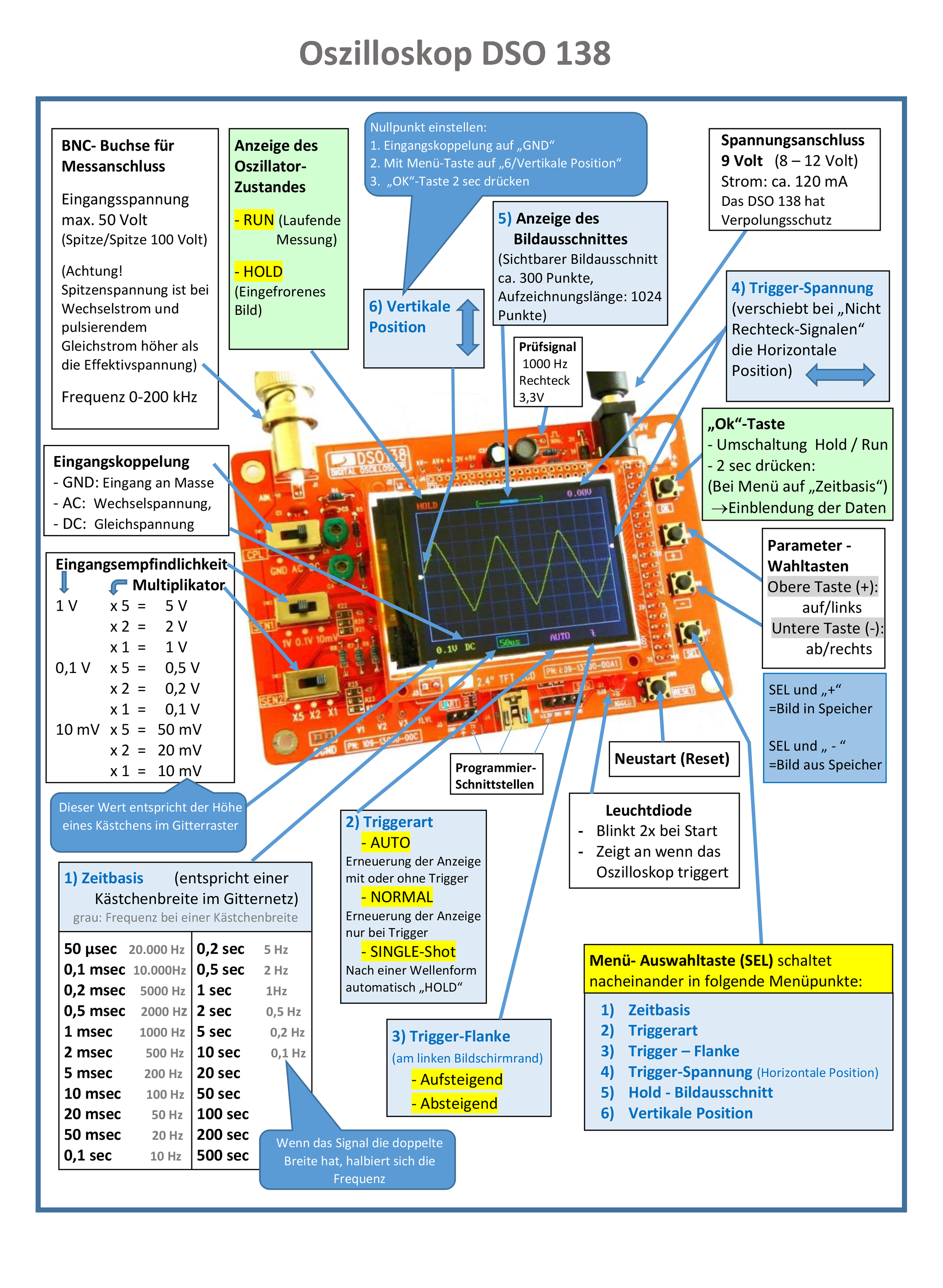
Quick Reference Guide

Assembly of the housing and commissioning

Power supply

You can get a power supply for about 10 euros in online shops. It is best to take a model with different adapters on the 9 V side, so there is certainly the right one. As mentioned earlier, battery operation also works. But even then you need the right adapter. I’ve crafted something for it:

Probe compensation

Each probe has a certain capacity. Although small, its effect is increasing at high frequencies and must be compensated. If, like me, you have a kit with a housing, then first do the probe compensation before you install the DSO 138 in the housing. Afterwards, the relevant parts for the compensation are not accessible anymore.

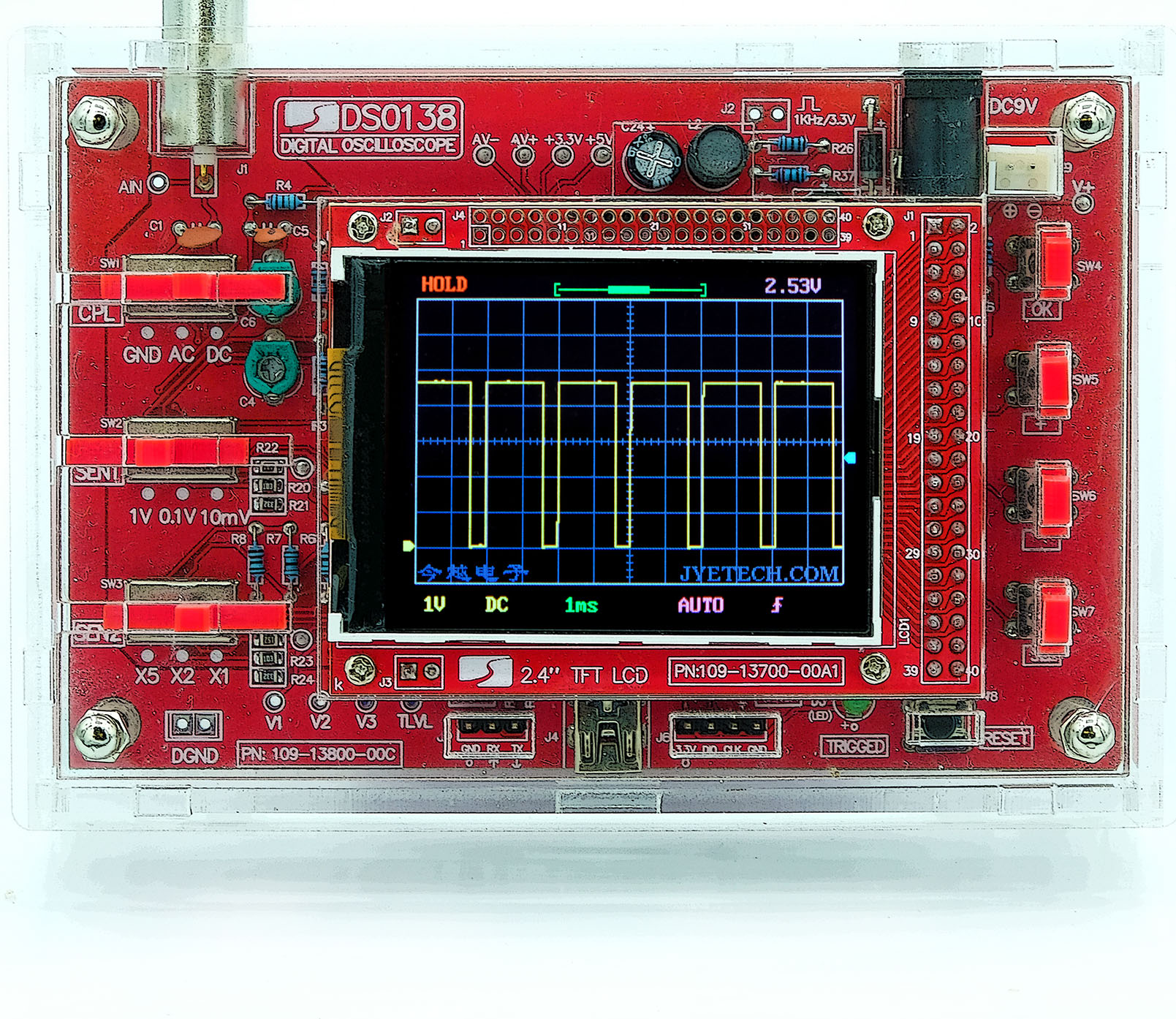
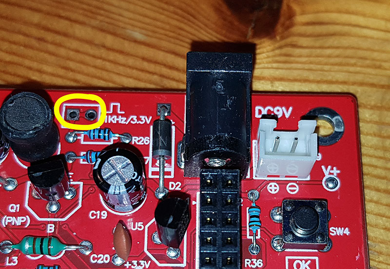
For calibration, the DSO 138 has an integrated 1 kHz / 3.3 V rectangular signal. To use it, however, you need to solder a wire bridge over the jumper highlighted in the image so that you can attach the crocodile clamp. Alternatively, you generate such a signal with the Arduino (see last post). Note: always connect GND (black cable) first for all measurements.

This is the procedure when using the internal signal:

1. Connect the red cable to the wire bridge (GND is internally connected in this particular case).
2. Set couple selection to AC or DC.
3. Select 0.1 Volt on the sensitivity slider 1.
4. Select X5 on the sensitivity slider 2.
5. Set time base to 0.2 ms.
6. Select auto mode. If there is no stable signal, then adjust the trigger level so that it is in the signal range.
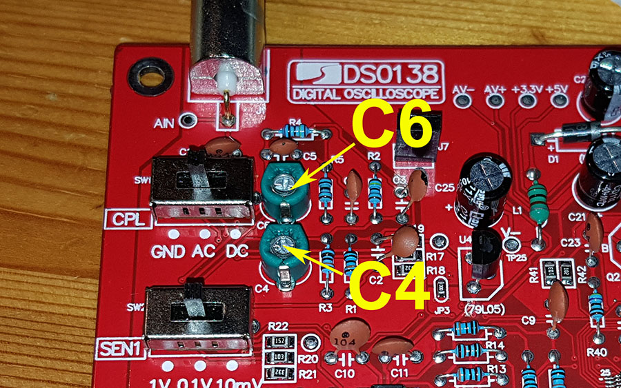
7. Adjust the capacitor trimmer C4 until you have beautiful rectangles (see below).
8. Now select 1 V on sensitivity 1 and X1 on sensitivity 2. All other settings remain the same.
9. Now adjust trimmer C6 till you have a perfect rectangle.

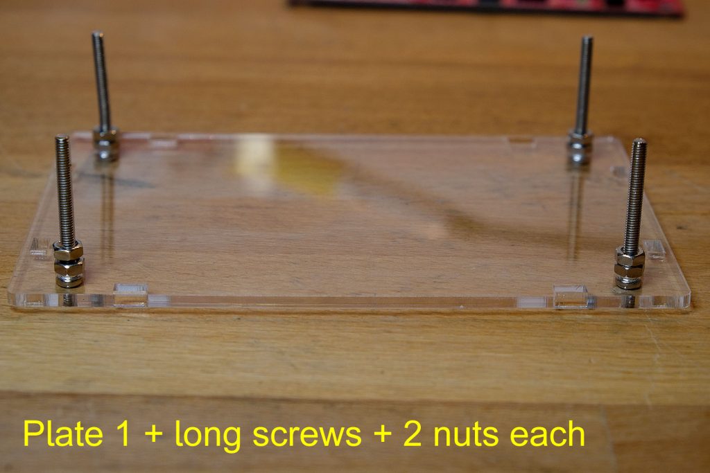
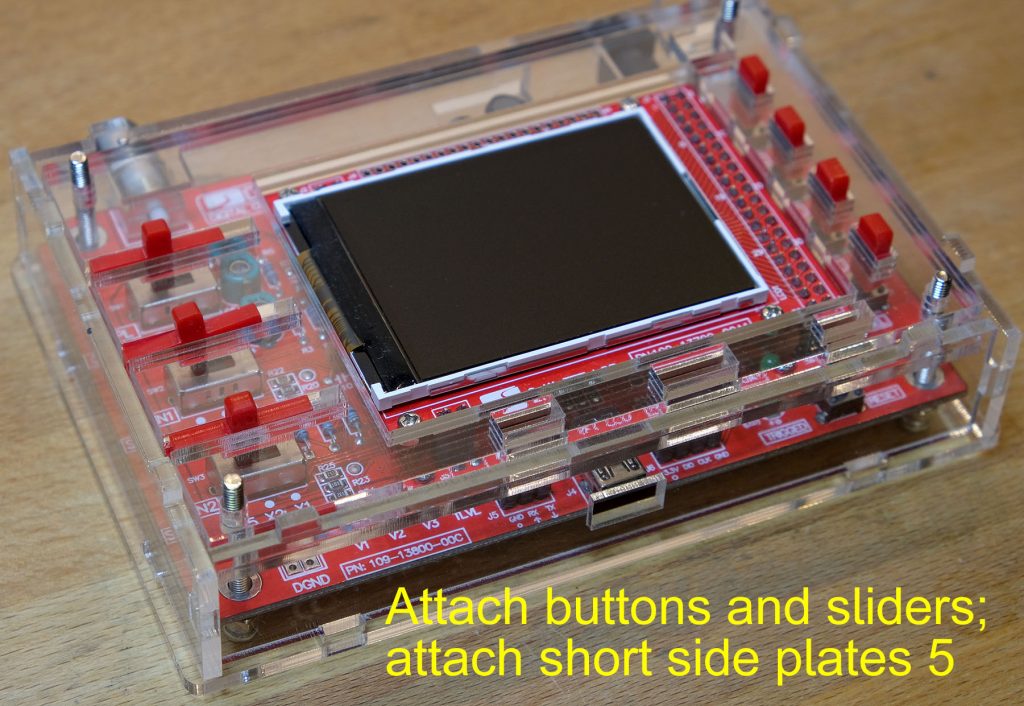
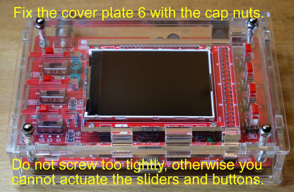
Mounting the housing

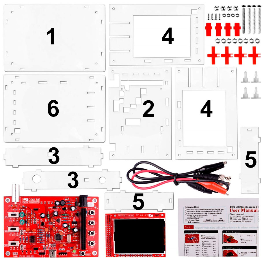
If you use the same housing as me, then maybe the instructions below will help you. First, you need to remove the protective film from the plexiglass components, the switches and the sliders. This is probably the most annoying part by far. Don’t forget to remove the protective film from the TFT display. You should not do the assembly in the dustiest place. I recommend wiping the table or workbench beforehand. Afterwards you get annoyed – I know what I’m talking about…

Trigger Modes

The trigger concept makes an oscilloscope reasonably usable in the first place, as it ensures a stable image. Only with very slow-changing signals triggers would be dispensable.

A trigger is an event in which a threshold (trigger level), i.e. a certain voltage level, is reached under consideration of the trigger slope. If the falling edge is defined as trigger slope, then there is a trigger when the trigger level is reached from top to bottom. With the rising edge, on the other hand, it is the other way around. Trigger mode determines the conditions under which a refresh screen is performed.

Auto Mode

In auto mode, screen refreshes are performed, whether there is a trigger or not. If there is a repeating signal trigger, the image is always updated at the same reference point. This makes the image stable. If there is no trigger, the screen is updated regularly, but at random points. This often looks as if the signal is moving through the screen. Just try it by applying a periodic signal and letting the trigger level move out of the signal level or into it.

Normal mode

In Normal Mode, the screen is only updated when there is a trigger. So if you push the trigger level out of the signal range, you’ll see how the screen refresh stops. If you push the trigger level back in, the screen refresh will start working again.

Single Mode

Even in single mode, there is no screen refresh if there is no trigger. If there is a trigger, the signal appears on the screen. But then the DSO 138 immediately goes into hold mode.

Single mode and normal mode are particularly suitable for single, rare or irregular signals.

So much for the theory. Play around a bit and things will become clearer quickly. But if you want to read a simple article about the operating modes again, then here is a link to it.

Practical examples

General comments

In the beginning you might need a few tries to conjure up a nice signal on the screen, but this gets faster and faster over time. If you know what voltage the signal will have maximum, then set the sensitivity accordingly. Set the trigger to approximately 50% of the expected signal. It doesn’t matter that much – most importantly it’s within the signal limits and outside the noise. Then modify the time base settings until the signal is stable and it uses the x-axis appropriately. Finally, you might make it even more beautiful by adjusting the vertical and horizontal position.

An analogWrite signal at the Arduino

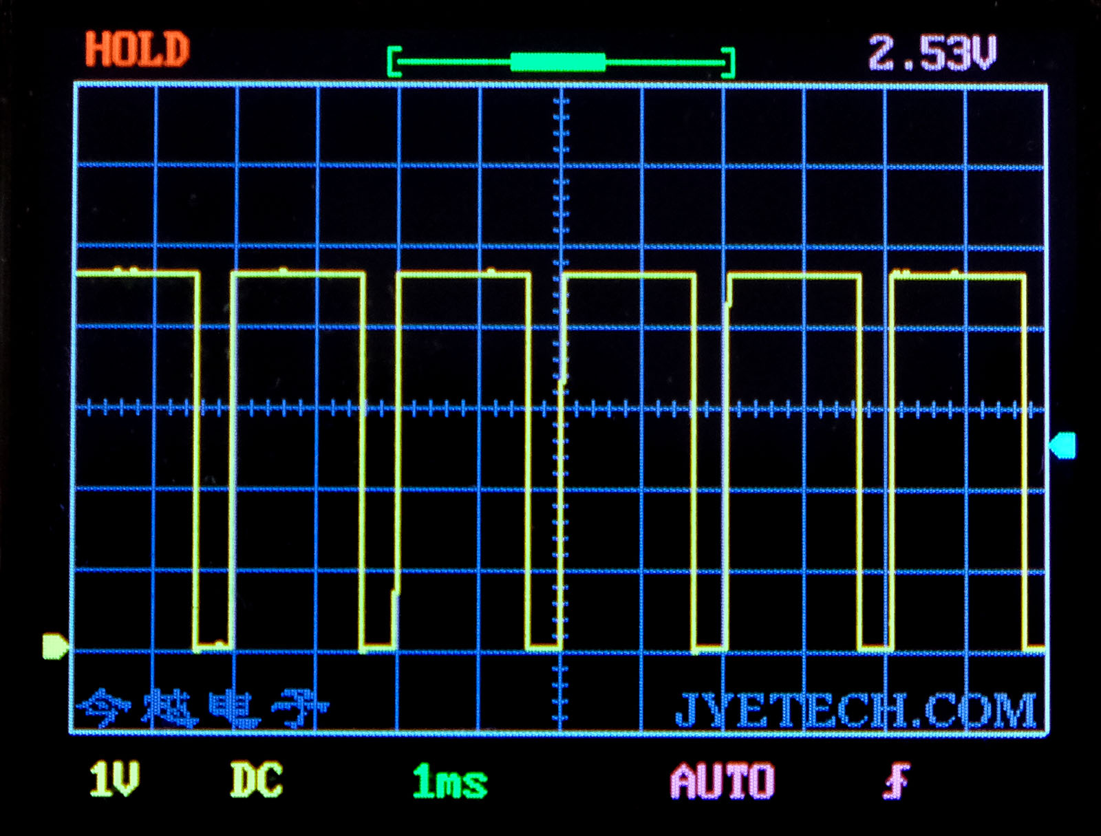
In the first example I created an analogWrite signal on the Arduino. As you can see, such an analogWrite signal is not really analogous, as it is generated via PWM (pulse width modulation).

Controlling a servo motor

Here I generated a control signal for 90° with the servo library. The frequency is detected correctly. At 90° the pulse width should be 0.0015 s, duty should be 7.5%. Duty is a bit too low (fluctuates on the display). Due to rounding and limited number of digits, the pulse width lands at 0.001 s. With a smaller time base, duty becomes more accurate and stable.

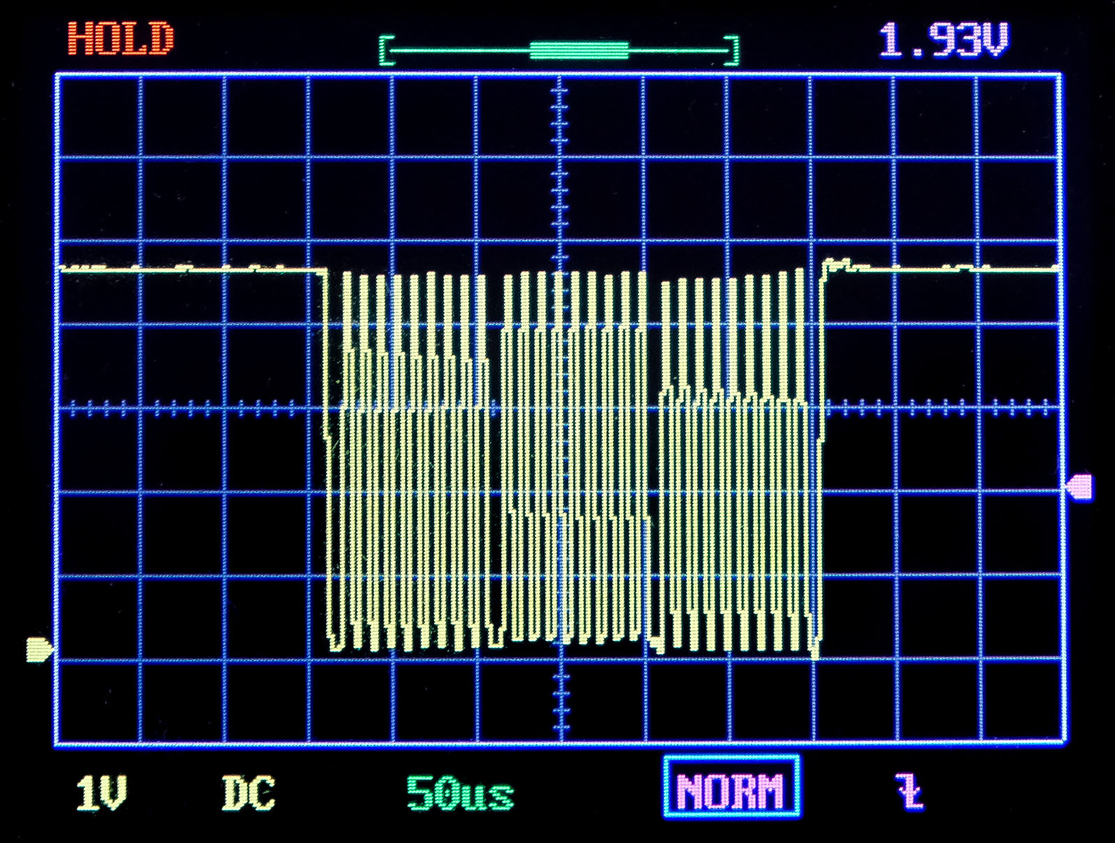
An infrared transmitter signal

Here I captured a signal from an infrared remote control (see also my article about this topic). As a non-periodic signal, this is a typical application for normal or single mode.

Signal of a 433 MHz handheld transmitter

This is again a task for normal or single mode. See also my posts about 433MHz hand transmitters and radio sockets and own radio protocols.

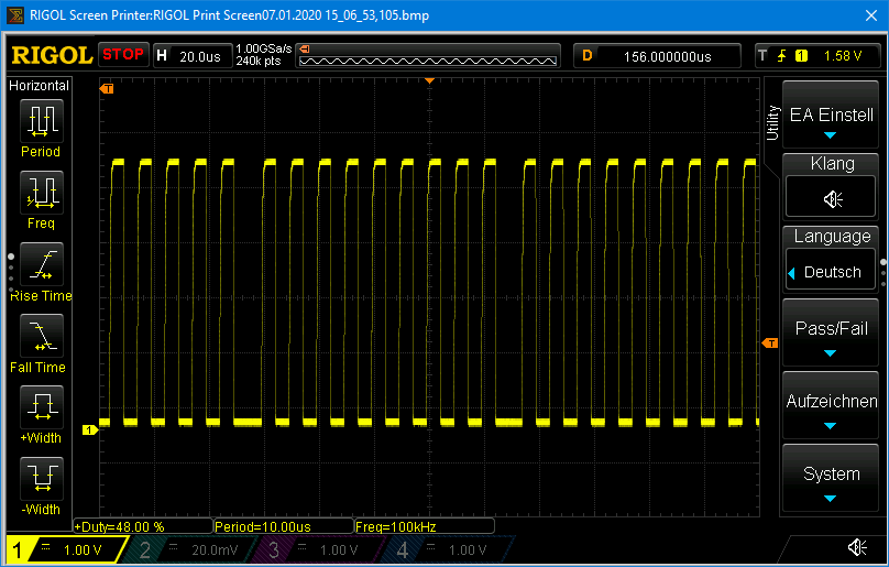
Limits of the DSO 138 using the example I2C

For this experiment, I controlled an I2C component with the Arduino and “intercepted” the SCK line signals with the oscilloscope. I chose the 100 kHz I2C mode because 400 kHz (fast mode) is resolved too poorly by the DSO 138. But even with 100 kHz we reach the limit. The signal cannot be resolved more finely. With a time base of 20 s, it disappears from the display.

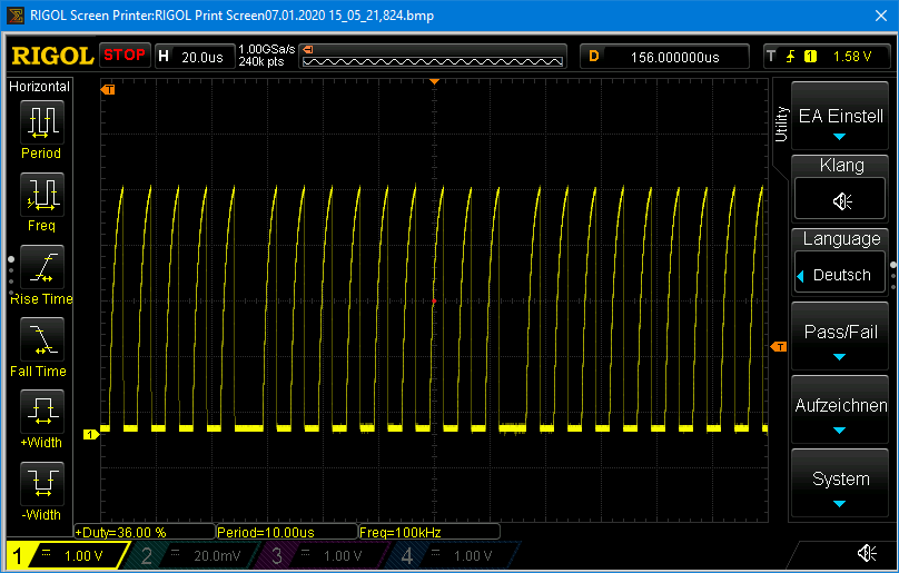
Then I took the pull-up resistance from the I2C clock line. The result is as it is:

You can see that the individual signal peaks are no longer as pronounced, but you cannot see what is happening in detail.

With my “good” oscilloscope, however, the measurements look like this:

Here you can clearly see how long it takes until the HIGH level is restored when no pull-up is used. That’s a big difference in the performance of the oscilloscopes – but this model costs more than ten times as much.